|
CS 294-2, Grouping and Recognition (Prof. Jitendra Malik) |
Oct 20, 1999 |
||
|
Lecture #16 (The figure/ground problem) |
Notes by Hector Magno |
||
This course is split into three parts: grouping, figure/ground, and recognition. Until now, every lecture has dealt with solving the grouping problem. Unfortunately, the figure/ground and recognition problems are not as well understood as the grouping problem (there are no good precise mathematical models for them). In fact, so little progress has been made on the figure/ground problem that we only spend one lecture on it. We plan to spend the rest of the semester on the recognition problem.
In this lecture, we explore the figure/ground problem in both natural images and images used in psychology studies. These notes are divided into the following three sections:
|
1. Introduction to the figure/ground problem 2. Rubin’s rules for distinguishing the figure from the ground 3. Traditional cues used in computer vision to solve the figure/ground problem |
1. Introduction to the figure/ground problem
The figure/ground problem is the problem of separating objects in the foreground from the background. This information can be used to determine the shape of objects in the image. For example, in the image below, it is clear that the tiger is the figure and the grass lies in the background:
In general, the figure/ground problem involves a depth ordering of the objects in the image. Keep in mind that it is possible for an object to act as both figure and background if there is an object in front of it and another one behind it. Hence, the figure/ground problem can be a quality local to parts of an image. To solve the figure/ground problem one must answer two questions:
1. Which object does the boundary curve belong to? The boundary curve should belong to the figure. So in the image above, the boundary between the tiger and the grass belongs to the tiger.
2. What part of the ground continues behind the figure? This means determining the amodal completion of the ground. In the image above, the amodal completion is the connection between the grass above the tiger and the grass below it.
2.
Rubin’s rules for distinguishing the figure from the groundBetween the years of 1915 and 1921, Rubin did about 80% of what has been done to solve the figure/ground problem today. He derived a series of rules that try to describe how the human visual system solves the problem. These rules are to be used statistically, since they are not always true. These rules can also conflict with each other, as is shown in some examples later in this section. As a result, the best way to use them is in a Bayesian framework, where all of the rules together can contribute to the result.
2.1 The figure is a familiar configuration
People tend to consider as the figure objects that they recognize. For example, in the first set of images, people generally recognize a pineapple, a horse, and a woman as the figures. However, in the second set, where the images are upside down, the results vary more because the familiar configuration is not as obvious.


2.2 Smaller entities are considered to be the figure
People tend to interpret small entities in an image as the figure itself rather than as the background as seen through a hole in the figure. This is illustrated in the image below:
2.3 Surrounded entities are considered to be the figure
Regions in an image that are completely surrounded by another region are usually interpreted to be in front. This case is similar to the case described above, and the image above demonstrates this point.
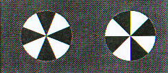
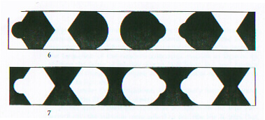
2.4 Objects that seem to be oriented vertically are interpreted as the figure
This rule is self-explanatory. The image below shows how it applies. Note that in the left picture, one tends to see a cross in front of a white background. This is not as obvious in the right picture, where the only factor that has changed is the orientation.
2.5 The figure is often symmetric
Because objects in nature tend to be symmetric, it is no surprise that symmetric objects tend to be considered the figure:
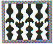
2.6 Convex objects are considered to be the figure
The mathematical definition of a convex shape is one where any two points that lie in the shape can be connected by a line that also lies completely in the shape. What complicates the application of this rule is that human beings use perceptual convexity, which is more flexible than the mathematical definition. Whereas the mathematical definition of a convex shape allows for clear-cut Boolean answers to the question of whether a shape is convex, the perceptual definition gives different degrees of convexity as answers. Unfortunately, there is no mathematical model for the perceptual definition. The images below illustrate this point:
Note that some of the objects that appear to be the figures are not exactly convex, but almost convex. Also note how this rule conflicts with the symmetry rule. This implies that this rule is stronger than the symmetry rule.
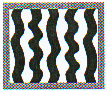
2.7 Parallelism of contours is a feature of the figure
This rule is closely tied with the symmetry rule. An example of this rule is shown below:
3. Traditional cues used in computer vision to solve the figure/ground problem
Of course, we are more interested in solving the figure/ground problem in more natural images than the ones shown above. This does not belittle the importance of Rubin’s rules, since they explain many of the cues that people use to solve the figure/ground problem. Nevertheless, there are other cues that are often seen in nature that can also be used. Such cues include T-junctions, terminators, texture information, and stereo/motion information.
3.1 T-junctions
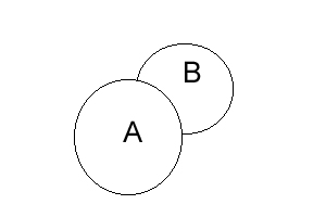
T-junctions are important because they arise when one opaque surface partially occludes another. This is a phenomenon seen often in nature, and people can easily label the figure from the ground in these scenarios.
|
|
Notice how in the figure on the left, region A clearly seems to be in front of region B. The intersection of the contours of the two regions forms a T-junction that implies this result. Note that T-junctions do not always lead to the right answer. T-junctions in textured regions are especially misleading. |
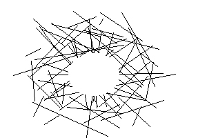
3.2 Terminators
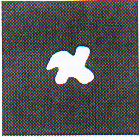
People are also good at connecting the ends of terminators to detect a figure that is partially camouflaged on a textured background. An example of this is shown below:
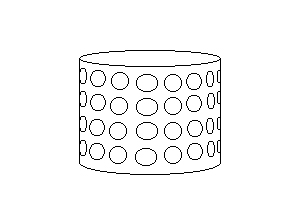
3.3 Texture information
Sometimes, the texture on a region can show the existence of an occluding contour, the contour that shows where an object curves around and hides itself. Such a contour easily points out the figure from the ground. Texture can point out such contours through the foreshortening effect. This effect causes the texture to change shape and appear more "squished" as it gets closer to the occluding contour. An example of this effect on a cylinder is illustrated below:
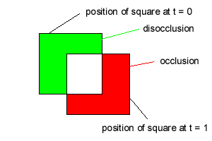
3.4 Stereo/motion information
The depth ordering of a scene can be directly derived from the disparity or optical flow information collected through stereo vision or observing motion. Moreover, the occlusion/disocclusion effect, also known as the accretion/deletion effect, also helps to distinguish the figure from the ground. This effect occurs in both stereo and motion, and it describes how parts of the background are hidden while other parts are revealed when the figure is moving or is seen from a different perspective. An example of this effect in the context of motion is shown below: